
Vector databases are the unsung heroes behind semantic search engines, AI chatbots with Retrieval-Augmented Generation (RAG), and smart recommendation systems. If you’re a developer (or an AI-savvy VP) exploring vector search solutions, this guide will walk you through Qdrant – a popular open-source vector database – in a comprehensive, code-focused way. We’ll cover what vector databases are, why Qdrant stands out, how to get started (with a few jokes to keep things light), and best practices for real-world applications. Let’s dive in!
Designing the retrieval layer end-to-end (chunking, embedding choice, hybrid search, evaluation) is the discipline we teach in Cohorte's Context Architecture course (E5).
Introduction to Vector Databases
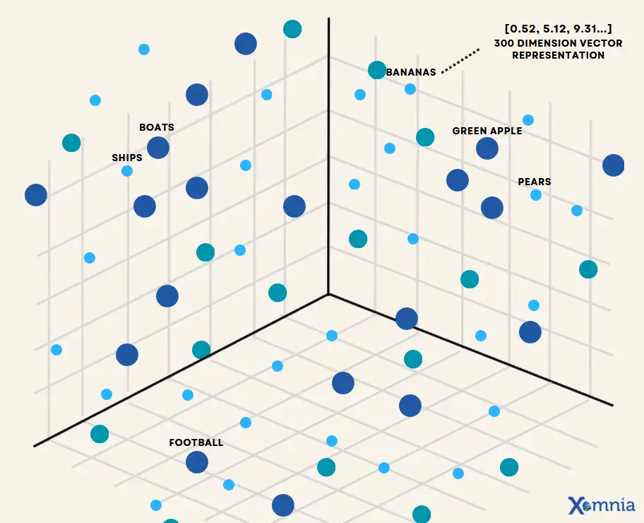
What on Earth is a vector database? In simple terms, it’s a specialized database for storing and querying vectors – numerical representations of data like text, images, or audio. Unlike traditional databases that retrieve data by exact matches or SQL conditions, vector DBs retrieve by similarity. You give the database a vector (e.g. an embedding of a search query), and it returns the items whose vectors are closest to it in the high-dimensional space. This unlocks semantic search (finding information based on meaning, not just keywords), recommendation systems (finding similar items/users), and RAG (Retrieval-Augmented Generation) pipelines for LLMs (fetching relevant context for a question). In essence, vector databases let AI applications retrieve data in a way that aligns with how AI models understand content – by meaning and similarity, not just exact text matches.
Traditional databases (SQL, NoSQL, etc.) struggle with this task – they aren’t optimized for the math of high-dimensional vectors. That’s why vector databases have emerged as a key component in modern AI stacks. They index vectors using algorithms like Approximate Nearest Neighbors (ANN) so that even searching among millions of vectors can be done in fractions of a second. Crucially, they often support filtering by metadata (like tags or categories) on those vectors, enabling queries like “find similar articles about climate change” (where “climate” is a filter on metadata).
In summary, vector databases matter in AI because they power:
- Semantic Search – e.g. searching documents by concept, not exact keywords (try asking your database for “JavaScript framework for front-end” and getting results about React/Vue without the exact words, thanks to embeddings).
- RAG Pipelines – retrieving relevant context paragraphs from a knowledge base to feed into an LLM (so the LLM’s answers are grounded in real data).
- Recommendations – matching user preferences to items (movies, products, memes – you name it) via vector similarity rather than predefined rules.
Now that we know what vector DBs do, let’s talk about Qdrant and why it’s a great choice in this space.
Why Qdrant?
There are many vector databases out there – so why choose Qdrant? Qdrant (pronounced “quadrant”) is a high-performance, open-source vector database written in Rust. It’s designed for real-time applications that need fast and accurate similarity search on large datasets. Here are some of Qdrant’s standout features and advantages:
- Speed and Performance: Qdrant uses the HNSW algorithm (Hierarchical Navigable Small World graphs) under the hood for ANN search, which is known for excellent performance on high-dimensional data. It’s optimized to handle millions of vectors efficiently, often achieving very high queries-per-second throughput in benchmarks. If your app can’t afford to keep users waiting, Qdrant’s focus on speed is a big win (it’s written in Rust, so you get C++-like performance with memory safety – no more “dangling pointers” ruining your day).
- Filtering & Hybrid Search: One of Qdrant’s superpowers is payload filtering. Each vector in Qdrant can have an associated JSON payload (metadata), and you can filter search results based on these fields without a big performance hit. Qdrant’s “filterable HNSW” means it builds indexes that respect your filters, so it doesn’t have to scan tons of results post-search. For example, you can ask for the nearest neighbors of a vector where
city="London", and Qdrant will efficiently return vectors only from London. It also supports hybrid search, combining vector similarity with keyword search by allowing sparse vectors (like TF-IDF or BM25 weights) in the same index. This gives you the best of both worlds: semantic matching + exact keyword matching when needed. - Flexible Integrations (API and Clients): Qdrant offers both RESTful HTTP API and gRPC API out of the box, plus client libraries in multiple languages (Python, TypeScript/JS, Go, Java, Rust, etc.) Whether you’re writing a quick Python script or building a high-throughput Go service, Qdrant has you covered. The Python client is particularly well-featured and even provides an embedded mode – you can run Qdrant in-memory inside your Python process for testing or small deployments. This embedded mode is super convenient: no need to stand up a server at all during development, just do
QdrantClient(":memory:")and go. - Open Source and Community: Qdrant is Apache-licensed and has a growing community (GitHub stars, active Discord). You get the freedom of open source with no vendor lock-in, and you can self-host it wherever you want – or use their managed cloud if you prefer. The project moves fast with new features (e.g. quantization for compression, distributed clustering, etc.) and performance improvements in each release. It’s a balanced choice for those who want “performance + flexibility + open-source freedom”.
- When does Qdrant shine? When you need a balance of top-notch performance, filtering, and ease of use. It’s great for use cases where speed and accuracy are paramount, such as real-time recommendations or anomaly detection on streaming data. Unlike some simpler libraries, Qdrant can handle dynamic data (adding/updating vectors on the fly) and still serve queries with low latency.
Of course, no solution is one-size-fits-all. We’ll later compare Qdrant to others like Postgres + PGVector, FAISS library, Weaviate, etc., and discuss when Qdrant might not be the best fit. (Spoiler: if you absolutely cannot run a separate service or you only need a tiny number of vectors in an existing SQL DB, alternatives might make sense. Otherwise, Qdrant’s likely a strong contender for production AI systems.)
Getting Started with Qdrant
Ready to try Qdrant? In this section, we’ll show you how to set up Qdrant both locally and via the cloud. Don’t worry – it’s easier than convincing an AI that “Phoenix” the city is not the same as “phoenix” the mythical bird.
Installing Qdrant
Locally (Docker): Qdrant provides a Docker image for easy deployment. Ensure you have Docker installed, then pull and run the Qdrant container:
# Pull the latest Qdrant image
docker pull qdrant/qdrant

# Run Qdrant with default ports (6333 for REST, 6334 for gRPC)
docker run -p 6333:6333 -p 6334:6334 \
    -v "$(pwd)/qdrant_storage:/qdrant/storage" \
    qdrant/qdrant
This will start Qdrant locally. It listens on localhost:6333 for REST and has a web-based UI at http://localhost:6333/dashboard for browsing your collectionsqdrant.techqdrant.tech. By default, data is stored in the mounted qdrant_storage folder on disk (so restarting the container doesn’t wipe your vectors). You can play with Qdrant’s nice Web UI to run test queries or inspect data if you like.
Qdrant Cloud: If you prefer a managed solution (or don’t want to install anything locally), Qdrant offers a SaaS cloud. You can spin up a free trial cluster on their Cloud web interfaceqdrant.tech. It’s as simple as creating an account, launching a cluster (e.g., on AWS or GCP regions provided), and grabbing the cluster URL and API key. We’ll use the local setup for examples (since it’s free and data stays on your machine), but using Qdrant Cloud with the Python client only requires passing the api_key and url to QdrantClient.
Python Client: Qdrant’s Python SDK makes it easy to interact with the DB. Install it via pip:
pip install qdrant-client(The client is open-source on PyPI. There’s also an optional [fastembed] extra that bundles a CPU-optimized embedding model, which we’ll touch on later.)
Once installed, you can initialize a client. If running Qdrant via Docker or Qdrant Cloud, you’ll connect by URL; for embedded mode, just give a path or use “:memory:”:
from qdrant_client import QdrantClient

# If using local Docker or remote Qdrant Cloud:
client = QdrantClient(url="http://localhost:6333")
# (For cloud, use url="https://YOUR_CLUSTER_URL", api_key="YOUR_API_KEY")

# If you want to run Qdrant in-process (no server needed, great for testing):
# client = QdrantClient(":memory:")  # in-memory
# client = QdrantClient(path="qdrant.embedded")  # persistent on disk file
Yes, you read that right: you can use Qdrant as a lightweight embedded database in a Python script with one line. It’s fantastic for unit tests or small apps – when you scale up, just point to a Qdrant server instead without changing your code.
Now that we have Qdrant up and running, let’s see how to use it with Python to manage collections and perform searches.
Using Qdrant with Python
We’ll go through the typical operations you’d do in a vector database: creating a collection, inserting vectors, querying for nearest matches, filtering by metadata, and updating or deleting data. All examples will use Python (since that’s common for AI workflows), but Qdrant’s concepts translate to other languages via their respective SDKs.
Creating a Collection
A collection in Qdrant is like a table in a relational DB – it holds a set of vectors (called “points” in Qdrant lingo) with the same configuration. When creating a collection, you specify the vector size (dimensionality) and the distance metric to use for similarity. Qdrant supports popular metrics: cosine, dot product, and Euclidean (L2) distance. You’ll typically choose the metric that matches how your embeddings were trained (e.g., if using cosine similarity in model training, use cosine in Qdrant).
Here’s how to create a new collection via the Python client:
from qdrant_client.models import Distance, VectorParams

# Create a collection named "my_collection" with 1536-dim vectors using cosine similarity
client.recreate_collection(
    collection_name="my_collection",
    vectors_config=VectorParams(size=1536, distance=Distance.COSINE)
)
We used recreate_collection which will drop the collection if it exists and make a fresh one – handy for demo purposes. In practice, you can use create_collection (which errors if the collection exists) or check for existence first. In this example, we assumed embeddings of length 1536 (which is common for OpenAI’s Ada 2 embeddings or certain SentenceTransformers). If your vectors are 768 or any other size, adjust accordingly. Qdrant collections are homogenous in vector dimension; it won’t let you insert a vector of a different length than specified – a nice safety checkairbyte.comairbyte.com.
By setting Distance.COSINE, similarity scores will be based on cosine similarity. Qdrant will internally normalize vectors if using cosine or dot for consistencyairbyte.com. (Normalization means you don’t have to worry if one vector is longer in magnitude; it treats all equally for cosine distance.)
Inserting Vectors (Points) and Payload
Now we have an empty collection. Let’s insert some vectors! In Qdrant, each vector (point) can have:
- an ID (unique per collection, either an integer or UUID),
- the vector embedding itself (an array of floats),
- an optional payload (a JSON-like dict of metadata, e.g. tags, text, etc.).
You can insert points individually or in batches. The Python client provides an upsert method that can add or update points. Let’s upsert a few points with some example data:
from qdrant_client.models import PointStruct

# Example vectors (e.g., embeddings of some texts) and payloads
vectors = [
    [0.05, 0.61, 0.76, 0.74],
    [0.19, 0.81, 0.75, 0.11],
    [0.36, 0.55, 0.47, 0.94],
]
payloads = [
    {"city": "Berlin", "country": "Germany"},
    {"city": "London", "country": "UK"},
    {"city": "Moscow", "country": "Russia"},
]

points = []
for i, (vec, meta) in enumerate(zip(vectors, payloads), start=1):
    points.append(PointStruct(id=i, vector=vec, payload=meta))

# Upsert points into the collection
result = client.upsert(
    collection_name="my_collection",
    points=points,
    wait=True  # wait for operation to complete
)
print(f"Inserted {len(points)} points. Status: {result.status}")
This will insert three points with IDs 1, 2, 3 and some payload fields. We included a simple payload with city and country just as an example of metadata. You could include any info relevant to your data: e.g. for documents, you might store {"title": "...", "url": "...", "text": "..."}; for images, maybe labels or creator info; for users/products, various attributes.
A few notes on inserting vectors:
- Qdrant supports batch inserts. In fact, the client’s
upload_pointsorupload_collectioncan take large lists and will internally batch them efficiently. Use these for big offline ingestion jobs (they callupsertunder the hood in chunks). - If you call
upserton an existing ID, Qdrant will update that point’s vector and payload (hence “upsert”). This is how you update vectors if your embeddings changed or you got new info for the item. - Qdrant is designed to handle large-scale inserts and even distributed ingestion (if running in cluster mode). Just keep an eye on memory if you insert millions in one go; batching and using
wait=Truein moderation helps.
Now that we have some data, let’s actually search for similar vectors!
Running a Similarity Search
Time for the fun part: querying for nearest neighbors. Typically, you’ll start with a new vector (for example, an embedding of a user query or an item) and ask Qdrant for the most similar points in the collection. Qdrant returns a list of scored points – each with an ID, the similarity score (or distance), and any payload if requested.
Let’s say we have a query vector [0.2, 0.1, 0.9, 0.7] (maybe an embedding of some query). We want the top 3 closest vectors we inserted:
# Query the collection for nearest neighbors of a given vector
query_vector = [0.2, 0.1, 0.9, 0.7]
results = client.search(
    collection_name="my_collection",
    query_vector=query_vector,
    limit=3,            # return 3 nearest points
    with_payload=True   # include payload data in results
)
for point in results:
    print(f"Found ID {point.id} with score {point.score}, payload={point.payload}")
When you run this, Qdrant will perform an ANN search in the collection and return, at most, 3 points. We set with_payload=True so we can see the metadata of the results. The score returned is the similarity score – for cosine or dot, higher is more similar; for Euclidean, lower means closer (Qdrant handles that behind the scenes).
In our small example, you’d get a list of points (IDs likely among 1,2,3) with their scores. For instance, if ID 4 was the closest, you might see something like:
Found ID 4 with score 1.362, payload=None
Found ID 1 with score 1.273, payload=None
Found ID 3 with score 1.208, payload=None(This sample output is from Qdrant’s docs with dot product metric, hence the scores. In our case with cosine, you’d get similarity values between -1 and 1.)
Under the hood, Qdrant traverses its HNSW index to find these near neighbors in sub-millisecond time for small data – and just a few milliseconds even if you have millions of vectors (depending on settings).
Adjusting search parameters: Qdrant allows tuning HNSW parameters like ef (the trade-off between speed and recall) if needed. For most cases, the defaults are fine (they aim to give ~95% recall). If you need absolutely exact results, Qdrant can do a brute-force search too, but that’s rarely needed once your index is built well.
Metadata Filtering in Queries
What if you don’t want all similar vectors, but only those matching some condition? For example, among similar items, you only want those in a certain category, or for a recommendation you want items the user hasn’t seen, etc. This is where Qdrant’s payload filtering comes in.
Let’s say from our earlier data, we want the nearest neighbor among vectors where city="London". We can add a filter to the search query:
from qdrant_client.models import Filter, FieldCondition, MatchValue

# Find nearest neighbors to the query_vector, but only where city == "London"
results = client.search(
    collection_name="my_collection",
    query_vector=query_vector,
    query_filter=Filter(
        must=[FieldCondition(key="city", match=MatchValue(value="London"))]
    ),
    limit=3,
    with_payload=True
)
for point in results:
    print(f"Found ID {point.id}, city={point.payload.get('city')}, score={point.score}")
Here we constructed a Filter that says: the point’s payload must have city matching "London". You can combine multiple conditions (the must list can have several, and there are also should and must_not for ORs and NOTs). Qdrant supports various conditions: exact match, range (> < >= <= for numeric), geo-bounding boxes, etc., on payload fields.
The result would print only points whose payload city is London. In our dummy data, that should retrieve the point with city London (ID 2) if it exists and is among the nearest. Indeed, Qdrant’s quickstart example shows that filtering by "London" returns ID 2 as the top result.
The beauty is Qdrant performs this filtering efficiently during the ANN search, thanks to its filterable index design. It doesn’t first fetch nearest neighbors from all cities and then throw away non-London ones (which would waste time) – instead, it traverses the index in a way that respects the filter. This means you can filter on millions of points with minimal overhead. Just remember to create payload indexes for fields you plan to filter on heavily (Qdrant can index payload values much like a traditional DB index to speed up filtering even more).
Updating and Deleting Vectors
By now, you’ve created a collection, inserted vectors, queried by similarity, and even filtered. But what about when your data changes? Applications often need to update vectors (perhaps re-embedding some text with a new model) or delete vectors (for instance, removing a discontinued product from recommendations).
Updating vectors: As mentioned, Qdrant treats any upsert of an existing ID as an update. So the simplest way to update a vector is to call upsert with the same ID and a new vector (and payload). If you only want to update the payload (metadata) without touching the vector, Qdrant provides client.set_payload to add/overwrite fields, or client.overwrite_payload to replace the whole payload. Similarly, there is client.update_vectors if you want to change just the vector for existing points without altering payload. These granular methods exist, but using upsert for full replace or set_payload for metadata is typically straightforward.
Example – updating payload for point ID 2:
# Update the payload of point ID 2 (say, correct the city name or add a new field)
client.set_payload(
    collection_name="my_collection",
    payload={"city": "London", "population": 9000000},  # maybe add population
    points=[2]
)
Example – updating the vector of point ID 2:
new_vector = [0.25, 0.8, 0.65, 0.2]  # new embedding for item 2
client.update_vector(
    collection_name="my_collection",
    points=[PointStruct(id=2, vector=new_vector)]
)
Under the hood, updating a vector will re-index that point. Updates are quite efficient for single points, but if you have to update many vectors (e.g. re-embed your entire dataset with a new model), it might be faster to rebuild a new collection or use bulk upload methods.
Deleting vectors: You can remove points by ID or by filter. The Python client’s delete method needs a points_selector to specify which points. For example, to delete by IDs:
from qdrant_client.models import PointIdsList

# Delete points with IDs 1 and 3 from the collection
client.delete(
    collection_name="my_collection",
    points_selector=PointIdsList(points=[1, 3]),
    wait=True
)
To delete by a filter (say, all vectors where country == "UK"):
from qdrant_client.models import Filter, FieldCondition, MatchValue, FilterSelector

client.delete(
    collection_name="my_collection",
    points_selector=FilterSelector(
        filter=Filter(must=[FieldCondition(key="country", match=MatchValue(value="UK"))])
    ),
    wait=True
)
The above would remove any point whose payload has country “UK”. Use this carefully! It’s powerful if you want to wipe segments of your data (e.g. delete all items of a category).
Deleting is generally fast – Qdrant just marks the point as deleted (and it won’t appear in searches). There’s also a concept of “soft delete vs hard delete” but by default the data is removed from the index. You can always insert new points with new IDs or reuse old IDs if needed.
That covers the CRUD operations on Qdrant. As you can see, the API is quite developer-friendly (and consistent – e.g., query vs search in the Python client, both exist but do similar things). Next, let’s explore some real-world use cases with Qdrant to solidify how it can be used in practical AI systems.
Real-World Use Cases
Qdrant isn’t just a toy for searching random numbers – it’s used in serious applications. Let’s look at a few common scenarios where Qdrant (and vector databases in general) excel, and how you’d implement them.
1. Semantic Search (Text Search on Steroids)
Scenario: You have a bunch of documents (articles, PDF content, support tickets, etc.) and you want to build a semantic search engine. Users will type questions or sentences, and you want to return the most relevant pieces of text, even if the words don’t exactly match.
How Qdrant helps: You’d embed all your documents (e.g. paragraph by paragraph) into vectors using a model like SentenceTransformers or OpenAI’s embeddings. Store those vectors in Qdrant with payloads that include the actual text and maybe metadata like title or source. When a user queries, embed the query text into a vector and use Qdrant to find the top-$k$ most similar document vectors. Then return those texts as search results.
Implementation outline:
- Data preparation: Split documents into chunks (to keep each embedding focused; chunking into, say, 100-300 word paragraphs is common). Compute vector embeddings for each chunk using a model. For example, using sentence_transformers in Python:
from sentence_transformers import SentenceTransformer
model = SentenceTransformer('all-MiniLM-L6-v2')
embeddings = model.encode(list_of_texts)  # returns a list of vector arrays
- Each embeddings[i] is a vector (e.g. 384 dimensions for MiniLM). Prepare payloads like {"doc_id": ..., "text": ..., "source": ...} for each.
- Index in Qdrant: Create a collection with the vector size (e.g. 384) and a suitable distance (cosine is popular for text embeddings). Use client.upload_collection to bulk insert all vectors with their payloads and IDs (maybe use the chunk index or a UUID as ID).
- Query time: Take the user’s query string, embed it with the same model to get a query vector. Call client.search(collection, query_vector=..., limit=10, with_payload=True) to get top 10 matching chunks. Each result comes with the original text (since you stored it in payload) and a similarity score.
- Display results: Show the text snippets to the user, perhaps highlighting the most relevant one. Because we used semantic similarity, the results might include texts that don’t contain the query words but are conceptually related – a big upgrade from keyword search.
Example: Suppose someone searches “benefits of solar panels” and your documents include a passage about “advantages of photovoltaic systems for renewable energy”. A keyword search might miss it if it doesn’t mention “solar” explicitly, but a vector search will likely catch it because “photovoltaic systems” is semantically similar to “solar panels”. Voilà – the user finds the right info.
With Qdrant, you can also add filters. Maybe the user only wants results from 2023 or later – if your payload has a year field, just add Filter(must=[FieldCondition(key="year", range=Range(gt=2022))]) to the search. Or if you have document categories, filter by category. This is extremely useful for narrowing down semantic search results by facets (date, author, type, etc.) without losing the semantic matching.
Qdrant’s ability to do hybrid search (dense + sparse) could also be applied here: you might combine the vector search score with a keyword search score. Qdrant 1.10+ has a new Query API to mix these signals, but even a simpler approach is to store a sparse vector of TF-IDF weights alongside the dense vector. Qdrant supports multiple vector fields per point (one dense, one sparse), and can perform a weighted sum of their distances. The result: your search can require that at least some important keywords match while still ranking by overall semantic similarity. This can improve result quality by avoiding off-topic but semantically loose matches (every vector search dev has seen the one odd result that’s conceptually similar but contextually irrelevant – hybrid search helps fix that by reining in the semantics with actual keywords).
2. Retrieval-Augmented Generation (RAG) with LLMs
Scenario: You’re building an AI Q&A bot or assistant that uses a large language model (LLM) like GPT-4 or Llama 2. You want it to provide accurate answers grounded in a knowledge base (docs, manuals, wikis) so it doesn’t hallucinate. This is the classic RAG setup – the LLM retrieves relevant info and then generates an answer.
How Qdrant helps: Qdrant will serve as the “knowledge store” of embeddings. You’ll embed all your knowledge base passages (similar to the semantic search above). Then at query time, before calling the LLM, you use Qdrant to fetch the top relevant passages for the user’s question. Those passages are fed into the LLM prompt (as context) so it can base its answer on them.
Implementation outline:
- Data ingestion: Suppose you have a company handbook PDF or a product documentation site. Use a pipeline (maybe with a tool like LangChain or LlamaIndex which have document loaders) to break into chunks and embed (using, say, OpenAI’s
text-embedding-ada-002which gives 1536-dim vectors). Store in Qdrant collection with payload containing the original text and maybe a reference (section/page). - User question handling: When a user asks a question, embed the question (with the same embedding model). Use Qdrant to search for, say, the top 5 most relevant chunks (use
client.searchwithlimit=5). Get those chunks’ text from the payload. - LLM Prompting: Construct a prompt for your LLM that includes the retrieved texts, e.g.: “Using the information below, answer the question: {question}\n\nRelevant excerpts:\n- Excerpt 1: {text1}\n- Excerpt 2: {text2}\n…”. Then ask the LLM to answer. The LLM will hopefully incorporate the provided facts in its answer, yielding a grounded response.
- Iterate as needed: If the answer isn’t sufficient, you could refine the query or fetch more from Qdrant. Some RAG systems also do a second vector search using parts of the initial answer to find more info (feedback loop). Qdrant can handle multiple queries very quickly so this is fine.
LangChain / LlamaIndex integrations: The good news is you don’t have to write all this from scratch. Libraries like LangChain and LlamaIndex have Qdrant integrations. For example, LangChain can use Qdrant as a VectorStore for its retrieval QA chain. LlamaIndex (formerly GPT Index) likewise can use Qdrant as the storage for indices. These integrations abstract away a lot of boilerplate: you’d just do something like VectorStoreIndex.from_vector_store(QdrantVectorStore(...)) and then ask questions to an index that automatically queries Qdrant. Under the hood it’s the same operations we described, but it’s nice to know the stack is compatible. So if your technical decision-makers are looking for “can we use Qdrant in our GPT-powered chatbot?”, the answer is a resounding yes – it plugs right in.
Bonus – real-time updates: If your knowledge source updates (new documents or data coming in), Qdrant can ingest those on the fly. You can upsert new chunks as they arrive, and they become immediately searchable. This is great for dynamic domains (e.g., pulling latest support tickets for an AI helpdesk, where you constantly add vectors). Just be mindful of vector consistency – if you retrain your embedding model or switch models, you’d want to re-embed existing data for best results (embedding space differences can mess up similarity). Qdrant doesn’t care, it will store whatever vectors you give, but that’s a user responsibility.
3. Recommendation Systems (User-Item Similarity)
Scenario: You want to recommend items to users (or content to readers, songs to listeners, etc.) based on similarity. One way is collaborative filtering via vectors: represent users by the vectors of things they like (or a learned embedding from their behavior) and represent items by feature vectors. Then find nearest neighbors – either find items close to a user’s vector (content-based recommendations) or find users similar to a given user to do “people like you also liked X”.
How Qdrant helps: Qdrant can store the vectors for all users and items and let you query across them efficiently. Thanks to metadata filters, you can even ensure, for example, you don’t recommend items the user has already seen by filtering those out, or limit to a certain category the user is interested in.
Implementation outline:
- Suppose you have item embeddings (maybe from a model or even something simple like word2vec on item descriptions) and user embeddings (perhaps an average of the embeddings of items they liked, or learned via matrix factorization or a neural model). Store all item vectors in a Qdrant collection with payload like
{"type": "item", "item_id": ..., "genre": "...", ...}. Store user vectors in the same collection or a separate one – Qdrant can handle either. Let’s assume one collection with a payload fieldtypethat is either"user"or"item". - To get recommendations for user X, you’d take user X’s embedding vector and do a similarity search in the collection for nearest neighbors with a filter
type="item"(so you only get items, not other users). This yields the closest items to the user’s preferences. You might further filter out items the user already interacted with by adding a filter condition likeitem_id not in {list_of_user_past_items}– Qdrant supportsmust_notconditions or a filter of list of IDs to exclude. - The result is a list of item IDs (with scores) to recommend. You can then fetch their details from your main database and present to the user.
Alternatively, you could do the reverse: store everything and filter differently. For example, to find “users similar to this user” (for a social app suggestion), you’d filter type="user" and query with that user’s vector to find neighbors. Or to find “items similar to item Y” (related products), query with item Y’s vector but filter type="item" to get other items.
Real-world note: Vector-based recommendations complement traditional collaborative filtering. They handle the “cold start” better if you have content information (you can recommend new items if their vector is similar to things a user likes, even if no one has liked the new item yet). And they capture nuanced relationships beyond exact co-occurrence. For example, a user who watched a lot of sci-fi movies might get a recommendation for a new sci-fi film that no similar user has watched yet, because the content embedding of that film is close to what they like. Qdrant’s fast search and filtering makes these scenarios feasible in real-time.
Also, Qdrant being real-time means you can update vectors as user tastes change or new items arrive. If a user suddenly starts listening to country music, you can adjust their vector (or add a new one for their recent preferences) and recommendations will shift accordingly.
4. (Bonus) Other use cases
While the prompt specifically asked for the above three, it’s worth mentioning Qdrant can be used anywhere you need similarity search:
- Anomaly Detection: Embed data points (transactions, telemetry, etc.) and find outliers by distance. Qdrant can quickly find the nearest neighbors of a new data point; if the distance to the nearest is above a threshold, it’s an outlier. Companies use this for fraud detection (as cited in Qdrant’s use cases).
- Multimedia search: Searching images by image (via embeddings from a CNN), searching audio by sound, etc. Qdrant doesn’t care if it’s text or images generating the vectors – you can store image embeddings and tag them, then query by an embedding of a new image to do “find similar images”.
- Hybrid filtering on user preferences: Qdrant’s payload filtering can implement things like “geographic radius search plus similarity” (store geo coordinates in payload, filter by a lat-long radius and do vector similarity on other features).
- Graph data as vectors: Sometimes knowledge graphs or graph embeddings are stored in Qdrant to enable finding related entities. Not a typical usage but an interesting one, combining structured graph relations with vector similarity.
The possibilities are vast – essentially any time you can represent something as a vector and you want to find similar ones, a vector DB is your friend.
Comparison with Other Vector Databases
It’s a booming field, and Qdrant isn’t alone. How does Qdrant stack up against some other popular vector search options? Let’s compare at a high level with PGVector, FAISS, Weaviate, and Chroma (all of which you might encounter in your vector DB shopping trips). We’ll look at factors like performance, filtering, scalability, and ease of use. And to keep things objective, we’ll include a little table for quick reference.
Qdrant vs. PGVector (Postgres extension)
PGVector is an extension that brings vector search to PostgreSQL. Its big selling point: you can use Postgres for vectors without a new system. If your data is already in a SQL database, adding PGVector means you can do SELECT ... ORDER BY vector <-> query LIMIT k right alongside your relational data.
- Performance: Generally, Qdrant as a specialized engine is faster for large vector corpora. It uses optimized indexes (HNSW) tailored for vectors, whereas PGVector initially did brute-force or IVFFlat indexing. Newer Postgres versions (15/16) have introduced HNSW and other indexing for PGVector, and there are reports of improved performance. However, independent benchmarks have shown Qdrant outperforming PGVector on throughput by a wide margin in many cases. Timescale (makers of TimescaleDB) published their own benchmark claiming PGVector could match or beat Qdrant at 99% recall with certain configurations – take that with a grain of salt as it likely involves specific tuning (and possibly their proprietary pgvectorscale). In general, for 99%+ recall (almost exact search), PGVector might do okay, but for extremely high-dimensional data at scale, Qdrant’s Rust performance and memory management usually shine.
- Filtering: PGVector relies on Postgres for filtering. That means it can filter on any SQL condition (very flexible), but it doesn’t integrate that into the index search the way Qdrant does. For example, you could do
... WHERE category='tech' ORDER BY embedding <-> query, but under the hood it may compute distance for many points then filter. With proper indexes on the category column and using Postgres query planner, it can be somewhat optimized, but Qdrant’s approach of combining filter + ANN in one step is purpose-built. So if fine-grained filtering with minimal latency is a need, Qdrant has an edge. - Scalability: Qdrant can scale horizontally using its distributed mode (sharding collections across nodes, plus replication) – it’s relatively new but available. With PGVector, scaling means scaling Postgres (which can be done via partitioning or using something like Citus). However, sharding a vector index across Postgres instances isn’t trivial, especially if you want ANN search across shards. You might end up doing something like query each shard then merge results, which increases latency. So for very large datasets (tens of millions+ vectors), Qdrant or other purpose-built systems are built with that scaling in mind, whereas PGVector remains single-node unless you add heavy extension magic.
- Ease of use: If you love SQL, PGVector is nice because you can stick to one database. No additional moving parts; backup and security piggyback on Postgres. However, using PGVector means writing SQL for vector search (which is okay but not as convenient as a Python client’s methods) and being mindful of Postgres config (shared memory, index build time, etc.). Qdrant’s API and clients are very straightforward for developers, but it’s an extra component to run. In an engineering hours calculation: integrating Qdrant might be a bit more work than a PG extension if your team is already very Postgres-savvy. On the flip side, if your use case outgrows what PGVector can handle, you’d spend far more time nursing Postgres.
When to choose PGVector: If your vector data is small to moderate (say, a few hundred thousand vectors) and you really want everything in one SQL database for simplicity, PGVector can be enough. It’s also a great way to prototype vector search in an environment you’re familiar with. Also, if your queries naturally join vector search results with relational data, doing it in Postgres might simplify the pipeline (no need to merge results from an external service).
When to choose Qdrant: When performance and scale are critical, or when you want advanced vector-specific features (HNSW tuning, product quantization, segmenting, etc.). Also, if you need easy client integration and not worry about writing SQL, Qdrant is nicer. For filtering heavy workloads, Qdrant will likely handle them more gracefully at large scale. In short, if you’re building an AI feature that is core to your product (and not just a tiny add-on), investing in a dedicated vector DB like Qdrant will pay off in reliability and speed.
Qdrant vs. FAISS (library)
FAISS (Facebook AI Similarity Search) is not a database but a C++/Python library for vector similarity. It’s extremely popular in the research community and underpins many bespoke solutions. You can think of FAISS as “roll your own vector store”: it gives you algorithms to index and search vectors in-memory.
- Performance: FAISS is highly optimized in C++ (with optional GPU support) and can be blazing fast. For pure ANN search on static data, FAISS often is the benchmark to beat. Qdrant’s engine is also in C++/Rust and uses HNSW (FAISS also offers HNSW as one of its index types), so performance is comparable for similar algorithms. But FAISS gives you more choices (IVF, PQ, etc.) to fine-tune speed/accuracy trade-offs. If you have billions of vectors and want to carefully optimize memory vs accuracy, FAISS is great as a library. Qdrant is catching up by adding features like quantization (vector compression) to also handle larger-than-memory scenarios, but FAISS is more mature in that realm.
- Features: The biggest difference – FAISS is just vectors. No payload storage, no filtering by metadata built-in Using FAISS, you’d get back just IDs of nearest neighbors, and then you must look up those IDs in your own data store to get the full info. Also, FAISS indexes are typically immutable after creation. You can add vectors, but you cannot easily delete or update individual ones (some index types allow add, but deletion is not straightforward). It’s meant for a static dataset that you build an index on, then query. No dynamic CRUD like Qdrant supports. If you need to update, often you have to rebuild the index.
- Scalability: FAISS is an in-memory library. It can handle large datasets (sharding is up to you to implement; some people partition by vector hash or train multiple indices). It doesn’t automatically distribute across machines – you’d have to do that logic. Qdrant, as a server, can use disk storage, and the upcoming/experimental distributed mode can spread data. Also, Qdrant can be queried while data is being inserted; FAISS usually expects you to finish indexing before querying for best performance.
- Ease of use: If you’re a Python or C++ developer comfortable with building indices and handling your own storage, FAISS is fine. But integrating it into a production service means you’re essentially writing your own vector database around it (to handle REST calls, or to manage ID-to-metadata mapping, etc.). Qdrant out-of-the-box gives you all that – a ready service with an API, persistence, metadata, etc. The developer experience of Qdrant is more plug-and-play (especially with the client libraries and cloud option), whereas FAISS is more DIY. It’s like the difference between using a database vs. using a sorted array and writing your own query engine.
When to choose FAISS: If you have a specialized scenario where maximal performance on static data is needed and you’re okay building some infrastructure around it. For example, if you’re doing an offline similarity search on a very large dataset to produce some analysis, FAISS might be ideal. Or if your application runs in a constrained environment (say, on-device) where you can’t run a server and need an embedded solution – FAISS could fit (though note: Qdrant’s embedded mode could also be used in some cases). Another case is if you want to avoid network calls entirely and keep everything in-process for latency reasons (microseconds matter).
When to choose Qdrant: For most application services where queries and updates happen online, Qdrant offers a lot more convenience and features. If you find yourself needing to implement features on top of FAISS that sound like “I need to store metadata” or “how do I delete points easily?” or “we need to serve this over HTTP to other services”, that’s a sign you’re re-inventing a vector DB. Qdrant (or another vector DB) will save you time here. Also, Qdrant supports filtering, whereas with FAISS you’d have to filter results post-hoc by checking IDs (which is slow if many results). Qdrant’s approach yields huge gains in such scenarios. In a nutshell, FAISS is great inside ML pipelines; Qdrant is great for production services.
Qdrant vs. Weaviate
Weaviate is another popular open-source vector database (written in Go). It distinguishes itself with a rich feature set: a GraphQL API, a built-in schema system, and “modules” that can do things like call external APIs for generating vectors (e.g. it can use OpenAI’s embeddings by just providing an API key, no separate code needed).
- Performance: Weaviate and Qdrant often go head-to-head in benchmarks. Both use HNSW for ANN. Anecdotally, Qdrant tends to be very slightly faster for pure vector search at times, but Weaviate is also highly optimized in Go. In the ANN Benchmarks and other tests, they’re usually in the same ballpark, with differences coming down to config and dataset. One independent benchmark showed Weaviate and Qdrant very close, with maybe Weaviate a tad slower on recall vs latency trade-offi. Both can do high QPS on large datasets, and both have options for multi-threading and such. Unless you push extreme scale, you likely won’t notice a major speed difference – they’re both “pretty fast”.
- Filtering: Weaviate supports filtering and hybrid search as well. It has an advanced schema where you define classes and properties, and you can filter on those properties (very similar concept to Qdrant’s payload filters). Weaviate’s query interface (GraphQL) allows specifying filters in queries. Under the hood, Weaviate also uses techniques to handle filters – I believe it also can use inverted indices for certain props. In short, both Qdrant and Weaviate were built with filter + vector use cases in mind and perform well there.
- Scalability: Weaviate offers a cloud service and also supports clustering (they have a concept of “sharding” data by class and “replicas”). One difference: Weaviate can dynamically scale out by sharding based on data properties or just automatically if using their cloud, whereas Qdrant’s distributed mode is newer and uses static sharding for now. Both can handle millions of vectors on a single node easily; for multi-node, Weaviate had it earlier, Qdrant is catching up. If you need multi-tenancy, both are adding features (Qdrant has a concept of clusters/namespaces, Weaviate has multi-tenancy at class level).
- Ease of use & Ecosystem: This is where they diverge more. Weaviate has a GraphQL API (and now also REST), and it strongly encourages you to define a schema for your data (like classes with fields). This is powerful if you treat Weaviate as not just a vector DB, but as a knowledge graph or database of record – you get data validation, a graph-like query language, etc. It even supports references between objects (so it can function somewhat like a graph DB + vector DB hybrid). Qdrant is schemaless in the sense that payload is just JSON, and you don’t define a formal schema upfront (beyond vector size/metric). That makes Qdrant more flexible and quick to start (no need to migrate schemas for simple changes), but Weaviate’s approach may be better for complex applications where you want the DB to enforce structure.
- Weaviate’s modules are a big plus: e.g., the “text2vec-transformers” or “text2vec-openai” modules let Weaviate handle calling an embedding model for you when you add data, so you can just send raw text and it stores the vector. Qdrant doesn’t do that on its own (though the Qdrant client’s
[fastembed]is moving in that direction by integrating an ONNX model for text embeddings). With Qdrant, you typically generate embeddings in your app code (or pipeline) and then upsert. With Weaviate, you could offload that to the DB (at the cost of some tight coupling to specific models). - In terms of installation, both can run via Docker easily. Weaviate historically had higher memory usage (it keeps a lot in RAM, especially for filters) – though it has improved with optional persistence and better memory control. Qdrant, being in Rust, often impresses people with a smaller memory footprint for similar tasks. There are anecdotal reports of Weaviate needing more resources for the same amount of data (especially if using text modules), so keep that in mind.
- Community & Support: Both have active communities. Weaviate BV (the company) and Qdrant (the company) are both very active in adding features. Weaviate had a head start on things like modules and a hosted cloud; Qdrant has been laser-focused on performance and core features. It’s a Coke vs Pepsi in some circles – many like Weaviate’s rich features, others prefer Qdrant’s simplicity and Rusty speed.
When to choose Weaviate: If your use case benefits from a strong schema (e.g. you’re basically building a knowledge graph with context) or you want one system that can also generate embeddings for you (less ML code in your app), Weaviate can be compelling. Also, if GraphQL fits better with your environment or you want to use the modular backend (like using Cohere’s API or built-in transformers without coding that yourself), Weaviate is unique in offering that. It’s also an all-in-one solution – you might rely on it as your primary data store for certain apps, whereas Qdrant is usually paired with another DB for non-vector data.
When to choose Qdrant: If you prioritize raw performance and a straightforward, no-frills approach. Qdrant’s simplicity (no need to predefine schema beyond vector size) can mean less upfront work. It also integrates easily into Python workflows (the Python client is very pythonic), whereas Weaviate’s Python client essentially wraps REST calls (which is fine, just a bit more verbose sometimes). If your team is more comfortable with REST/gRPC or you want to avoid GraphQL, Qdrant is the choice. Additionally, for purely vector-heavy workloads where you don’t need the extra bells and whistles of Weaviate, Qdrant might be lighter weight. It’s also worth noting that Qdrant’s filterable HNSW implementation is state-of-the-art; Weaviate uses HNSW + some tricks but might in some cases fall back to post-filtering depending on the query. Qdrant explicitly built their index to handle filtering first-phase, which could give it an edge for very complex filters.
Qdrant vs. Chroma
Chroma is a newcomer (open-source, in Python) that has gained a lot of traction especially among developers building prototypes and LLM apps. It markets itself as the “AI-native” vector store and is very easy to integrate in Python environments (it’s the default for LangChain’s quickstart, for example).
- Performance: Chroma, being implemented in Python (with some heavy lifting in NumPy/BLAS), is not as high-performance as Qdrant for large data. It’s fine for smaller sets (thousands to maybe low millions of vectors, depending on memory). Chroma often keeps everything in memory (it can use disk but initially had an in-memory SQLite meta store). It uses an HNSW (via
hnswlibunder the hood, I believe) for the ANN part, so raw search speed is decent. But overhead of Python and the fact that it runs in-process can show when you scale up or have concurrent queries. There have been reports of memory leaks or high memory usage and even crashes under load – as of late 2023, many of those are being addressed, but it indicates Chroma is still maturing. - Filtering: Chroma supports filtering on metadata to some extent (since it has a SQLite or DuckDB to manage metadata, you can do query like
.query(..., where={"author": "Alice"})). However, the filtering might not be as integrated with the ANN search as Qdrant’s. Likely it filters the set of candidates post ANN or uses some SQLite index to pre-filter candidates. It’s usable for simple equality filters, but it’s not a core strength. Complex filters or large cardinality might be slow. Meanwhile, Qdrant was built with filtering from day one. - Scalability: Chroma currently is primarily single-process. There is no sharding or multi-node support (unless you DIY it). It’s meant to be run as part of your application. They have plans for a client-server mode (which may be out by 2025, possibly making it more like Qdrant/Weaviate), but originally it was embedded only. That limits how much data you can handle (you’re constrained by the machine’s memory and Python’s performance). Qdrant, being a separate server in Rust with better memory management and optional distributed, will handle bigger scale more gracefully.
- Ease of use: This is Chroma’s forte. For a developer just wanting to add some semantic search to an app, Chroma is dead simple.
pip install chromadb, and a few lines to add data and query. It doesn’t require running a database server separately (just like SQLite is easy). It also has nice abstractions for collections and persistent storage (to disk) without much config. It even can manage embedding generation if you use theiradd_textswith an embedding function. In many tutorials for LLM QA, Chroma is the go-to for quick demos – it just works out of the box in a notebook. Qdrant, while also easy, does have that extra step of running a service or using the client’s local mode. But Qdrant’s local mode actually makes it comparable – you could argueQdrantClient(":memory:")is as easy as Chroma’s in-process usage. Still, Chroma’s Python-centric design (and being written in Python) means if you need to hack something, you can – it’s all there in Python code. Qdrant is a black box binary by comparison (though open source). - Features: Chroma has been adding features like
query_score(to get raw distances),persistetc., but it’s relatively minimal compared to Qdrant. No advanced indexing options, no explicit optimization settings exposed (like ef, M parameters). It aims for sane defaults for developers. Qdrant offers more control (which also means more to learn if you want to tweak). Chroma does have an interesting feature: you can dowhere_documentorwhere_metadataqueries easily, which is basically filtering. But as said, heavy use of that might hit Python limits.
When to choose Chroma: If you are in the prototyping stage or building a smaller-scale application in Python where simplicity trumps raw performance. For example, a personal project, a demo, or an internal tool with moderate data – Chroma gets you up and running fastest. Also, if you want everything inside a single Python app (maybe a Streamlit app doing QA), Chroma is convenient – no external service to deploy. It’s basically the SQLite of vector DBs in that sense: easy and sufficient for a lot of lightweight use cases.
When to choose Qdrant: When you need to move to production or handle larger scale/reliability. If your application might grow beyond a single process or you need concurrency and fault tolerance, Qdrant as a robust server makes more sense. Also, if you’re not limited to Python – e.g. your backend is in Node or Java – Qdrant provides a way to use vector search via its APIs, whereas Chroma (until it has a server mode) is locked to Python. For long-term projects, Qdrant’s stronger consistency (tested engine) might save headaches down the line. Essentially, start with Chroma if it fits, but be ready to switch to Qdrant (or another) if you hit limits. Many teams do just that: prototype with Chroma, then graduate to Qdrant for production.
To summarize this section, here’s a quick comparison table:
| Feature | Qdrant (Rust) | PGVector (Postgres ext) | FAISS (C++ lib) | Weaviate (Go) | Chroma (Python) |
|---|---|---|---|---|---|
| Open Source | Yes [source] | Yes (extension) [source] | Yes (library) | Yes [source] | Yes [source] |
| Hosting | Self-host or Qdrant Cloud [source] | Self-host (Postgres extension) | In-app library (no server) | Self-host or Weaviate Cloud | In-app library (server mode WIP) |
| Language/Stack | Rust server; multi-language clients | C/Postgres extension | C++ with Python bindings | Go with GraphQL/REST API | Python with SQLite/duckdb |
| Vector Index | HNSW [source] | IVF, Flat, HNSW (Postgres 16+) | HNSW, IVF, PQ, etc. | HNSW | HNSW (via hnswlib) |
| Metadata Filtering | Yes [source] | Yes – via SQL WHERE | No [source] | Yes – GraphQL filters | Basic (Python-side) |
| CRUD (Updates/Deletes) | Yes [source] | Yes – via SQL (expensive index rebuilds) | Limited [source] | Yes | Yes – but slower for heavy updates |
| Scalability | Cluster-ready (shards & replicas) | Single node (Postgres scaling) | No auto-scaling (manual shard) | Cluster-ready | Single node only |
| Performance (QPS/Latency) | Very high [source] | Moderate [source] | Extremely high (in-memory) | Very high | Moderate (Python overhead) |
| Ease of Use | High – simple APIs | High – if SQL fluent | Moderate – dev-focused | Moderate – schema setup required | Very high – Python-native |
| Unique Strengths | Filterable search, snapshots, client-side embedding | Uses full Postgres stack (ACID, joins) | Fine-tuned control, GPU support | GraphQL schema, knowledge-graph style | Quick prototyping, LangChain-ready |
| Potential Drawbacks | Extra service layer, no built-in embedding | Postgres load, lacks ANN optimizations | No server, no metadata, static index | Complex schema, higher memory use | Python-only, immature, bugs reported [source] |
As you can see, each option has its niche. Qdrant positions itself as a strong general-purpose solution – great performance, filtering, and ease, without locking you into a specific tech stack (since it’s language-agnostic via REST/gRPC). If you need a quick local solution in Python, Chroma might be enough. If you want one database for everything and vector search is a side feature, PGVector could work. If you’re building something like a semantic CMS or knowledge graph with complex schema, Weaviate offers a lot. And if you’re a research engineer who wants to squeeze every last drop of performance and doesn’t need a “database service”, FAISS is formidable.
Performance Tips & Best Practices
No matter which vector DB you choose, there are best practices to get the most out of it. Here are some tips particularly for Qdrant (though they apply broadly):
- Choose the Right Dimension & Model: The vector dimensionality affects speed and memory. Higher dims = slower queries and more space per vector. Don’t use a 1536-dim model if a 384-dim one works just as well for your task. It’s a trade-off between representation power and efficiency. Qdrant can handle high dims, but you’ll get more QPS from 384-d vectors than 1536-d given the same hardware.
- Chunk Your Data: For text, chunking documents into smaller passages not only improves semantic search relevance (you avoid diluting context), but also yields more, smaller vectors that are faster to index and search. It’s better to have 10k vectors of length 100 than 1k vectors of length 1000 words in many cases, in terms of both accuracy and performance (because shorter chunks embed to vectors that are easier to match precisely). Just don’t go too small or you lose meaning – find a sweet spot for your domain (commonly 50-300 words per chunk for docs).
- Batch Operations: When indexing, use Qdrant’s batch upload capabilities. For instance,
client.upload_collectionwill batch internally to avoid overwhelming memory If using upsert in a loop, consider chunking your calls (e.g., insert 1000 points at a time). This significantly speeds up loading. Also, usewait=Truejudiciously – you might not need to wait on every batch, maybe every Nth batch or at the end. - Indexing Parameters: Qdrant’s HNSW index has settings like
M(graph connectivity) andef_construct(depth of neighbor search during index build). The defaults are chosen well for most, but if you need faster queries and can tolerate slightly lower recall, you can loweref_search(theefused during search) oref_construct. Conversely, if you want higher recall, increaseef_searchat query time (the Python client’s search has a param for that). There’s also anexactsearch mode if needed for small data or debugging – but avoid it at large scale except for ground-truth comparison, because exact search doesn’t use ANN and will be slower. - Hybrid Search Strategies: If doing hybrid (dense + sparse), consider normalizing the scores of each or using a simple weighted sum. Qdrant 1.10 introduced a robust way to do this by composing multiple “should” clauses (one for vector similarity, one for keyword) in a single query DSL. For example, you might require a keyword match (sparse vector dot > 0 for that word) and then among those, rank by dense vector similarity. Experiment with what yields the best result quality.
- Memory Management: Qdrant stores vectors on disk by default, but will memory-map them. Ensure your machine has enough RAM for the index (or at least enough for the portion of index frequently accessed). Use payload indexes for fields you filter on often – Qdrant can create a structured index (like b-tree or inverted index) on payload data to speed up filters. This can dramatically improve filtered query latency and reduce CPU usage, at the cost of some RAM to hold the index.
- Parallelism and Throughput: Qdrant will utilize multiple threads for searching if you ask it to (by default, the number of threads might equal the number of CPU cores). If you have heavy concurrent load, tune the thread pool or consider clustering. For read-heavy scenarios, Qdrant’s async I/O (especially with the Rust client or gRPC) can help maximize throughput. The Python client is synchronous by default, but you can use the REST API asynchronously or the
grpcinterface for high QPS use cases (or just run multiple instances of your querying service, since Qdrant itself can handle concurrent connections). - Use IDs and Payloads Wisely: Storing huge blobs of text in payload might bloat the DB (and slow down network responses when you get results). It’s often better to store an identifier and perhaps a short snippet, then use the ID to fetch full data from a separate store (like an object storage or a database). For example, store
doc_idand maybe a summary sentence in Qdrant, then retrieve the full article text from S3 or a cache when needed. Qdrant is not meant to be a large blob storage – it’s fine with kilobytes of JSON per point, but don’t try to stuff entire PDFs in the payload. - Monitoring and Maintenance: Keep an eye on Qdrant’s telemetry if available. Monitor search latency and index size. Qdrant allows creating snapshots of your collections – use this for backups. Also, as you update/delete data, consider periodic index optimization (compactification). Qdrant may fragment data on disk after many deletions; currently, I believe one has to recreate collection or so to compact, but this may improve. Plan for re-indexing if you swap embedding models entirely (no vector DB magically makes two different embedding spaces directly comparable).
- Security: If deploying Qdrant in production, use its security features – Qdrant Cloud provides encryption and authentication keys. For self-host, you might want to run it behind a firewall or use an API gateway with auth, since Qdrant’s open-source version (as of now) doesn’t have role-based access or authentication built-in (it’s expected to be run in a protected environment or with a reverse proxy adding auth). Always secure your vector database if it contains sensitive data – just because it’s vectors doesn’t mean they aren’t sensitive (vectors can be inverted to approximate original data in some cases).
- Stay Updated: The vector DB field is evolving fast. New versions of Qdrant bring significant improvements (e.g., Qdrant added quantization support which can compress vectors to reduce memory by 4x or more with minimal accuracy loss – useful if you have massive datasets). Also keep an eye on competitors; it’s good to know what’s out there as techniques cross-pollinate (for instance, if a new ANN algorithm outperforms HNSW, Qdrant or others might adopt it).
Following these practices will help ensure your Qdrant-based system runs smoothly and efficiently. It’s always a good idea to test with your specific workload – e.g., simulate queries you expect in production and measure Qdrant’s performance, try different limit values (searching top 100 vs top 10 can have slightly different optimal settings), etc. The defaults are great, but a bit of tuning can go a long way for extreme cases.
Closing Thoughts
Qdrant is a powerful addition to the AI developer’s toolkit. It shines when you need a production-ready vector search engine that’s fast, filterable, and friendly to integrate. We’ve seen how it can be used for semantic search, LLM augmentation, recommendations, and more. Its strengths lie in performance (thanks Rust!), flexibility (payloads and filters), and an accessible API for developers. Being open-source doesn’t hurt either – you can run it anywhere and avoid hefty vendor fees (its cloud is optional and reasonably priced, with even a free tier for small projects).
So, when is Qdrant the best fit? When your application demands semantic understanding of data at scale. If you’re building a feature where relevant results matter more than exact keyword matches – whether it’s a smart search bar, a personalized feed, or an AI assistant that actually cites sources – Qdrant provides the backbone to make it happen. It’s particularly great if you need to combine vector similarity with other conditions (like time ranges, user preferences, etc.) due to its advanced filtering. And if you appreciate solid engineering, Qdrant’s design (Rust, embeddable, high-performance) is quite appealing.
And when might Qdrant not be ideal? If your use case is very small or simple, and you don’t want any external service, an embedded library like Chroma or even just brute-force search might suffice. If you have an existing relational setup and only a light vector need, PGVector inside Postgres could be easier to start with. If you require online learning or frequently updating a billion-vector index with strict real-time constraints, you might explore specialized solutions (though Qdrant can handle a lot, extremely high update rates might favor something like Milvus with GPU indexing, or an approximate approach where you rebuild index nightly). Also, Qdrant’s focus is vectors – if you wanted a one-stop solution that also handles your non-vector data with complex transactions, Qdrant won’t do that (you’d pair it with a SQL/NoSQL DB). And while Qdrant is adding enterprise features, if you need things like role-based security within the DB and you’re not comfortable adding a proxy or using cloud, a solution like Pinecone (fully managed with user management) might tick that box – albeit at significant cost and loss of open-source freedom.
In our experience, though, Qdrant is a fantastic middle ground for most vector search needs: more robust and feature-rich than a bare library, but lighter-weight and more developer-centric than some heavy “AI databases.” It has a bright future with the rapid growth of AI applications. Whether you’re an engineer implementing a similarity search or a technical leader evaluating options, Qdrant is definitely worth a try. Plus, nothing beats the satisfaction of querying a database by meaning and getting results that make you go “Whoa, the AI actually understood that!” 🤖🎉
Empathetic Parting Words: Embracing vector databases might feel like a leap if you come from the cozy world of SQL or the wild west of NoSQL. But remember, it’s addressing a need that those couldn’t: understanding unstructured data. It’s okay if at first you find yourself Googling “cosine similarity” or scratching your head at why your 768-dim embeddings aren’t returning perfect results – we’ve all been there. The good news is, tools like Qdrant abstract away a lot of the hard stuff, letting you focus on building the fun stuff (like that AI feature that will make your app 10x cooler 😎). And hey, if your first implementation isn’t perfect, just iterate – tweak your model, adjust your queries, and soon you’ll wonder how you ever lived without vector search.
Happy coding, and may your vectors always find their nearest neighbors!
Tega AdeyemiMay 13, 2025